Contribution to sea level rise
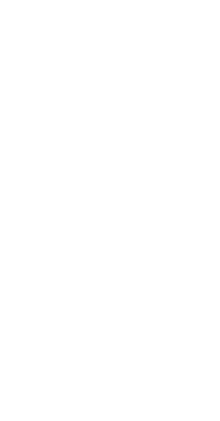
The contribution of ice caps to sea level rise is essentially a combination of three phenomena: snowfalls and melting of ice on the surface, due to climate change and variations in glacier altitude; thinning of floating ice shelves, which are melting from below because the ocean is warming up; and the discharge of ice into the sea when ice flowing towards the sea breaks off, calving icebergs.
Modelling and simulation
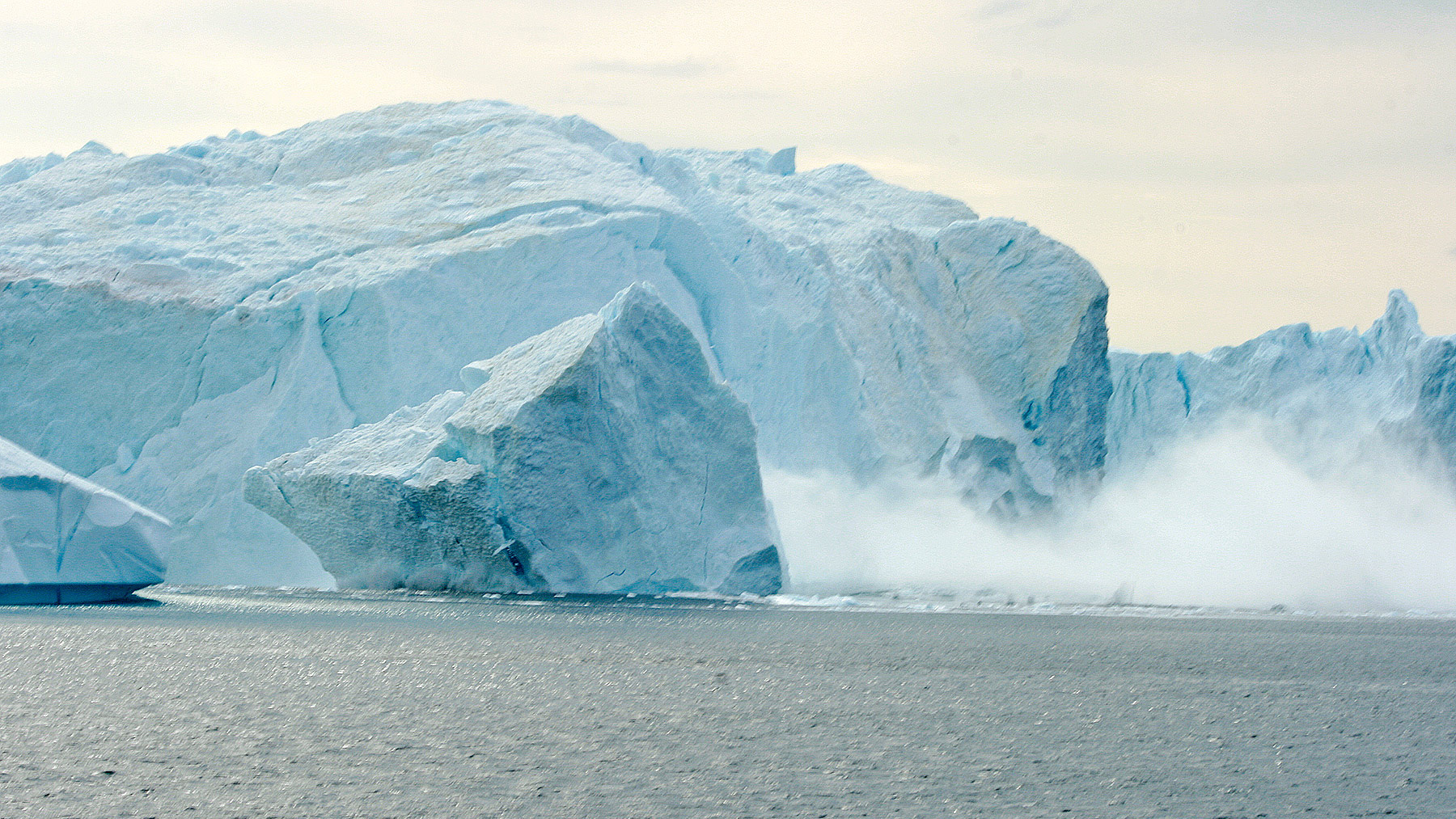
 Subglacial river frozen in winter
Photo : Yves Chaux
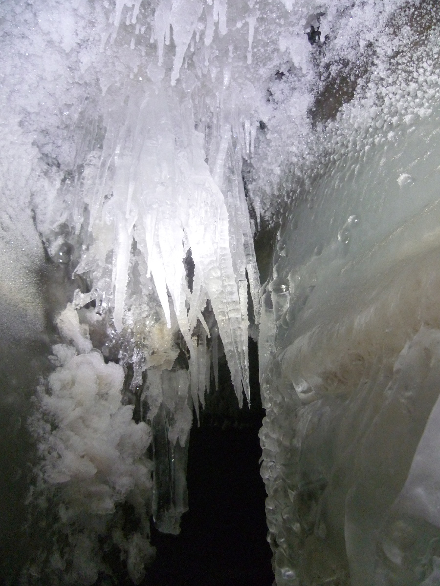
 Snow-covered surface of a glacier
Photo : Yves Chaux
The physical processes in an ice cap, both inside and on the surface, are being studied by glaciologists, in collaboration with climatologists, oceanologists, mathematicians and computer scientists. A numerical model based on mathematical equations can be used to simulate the ice cap dynamics, particularly the calving of icebergs. Algorithms solve the equations and are used in the computer codes.
Physical processes at work in an ice sheet
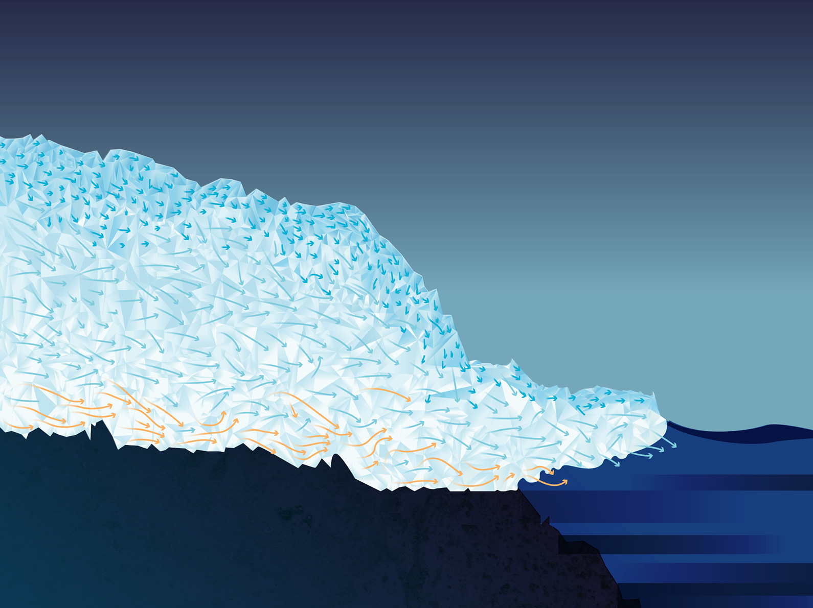
Inside
Ice is a fluid that flows under the influence of gravity. It flows much more slowly than liquid water because it has different characteristics. In particular, ice is a plastic fluid, i.e. it changes shape when it flows. The physical and mechanical properties of ice change with pressure and temperature. Pressure increases with depth because of the weight of the ice, and temperature, which is very low on the surface, also increases with depth. Consequently, the velocity of the glacier varies in intensity and direction inside the ice cap.
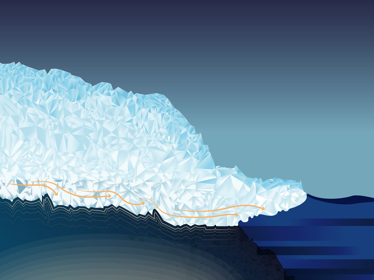
At the base
When the ice is cold, at the base it sticks to the bedrock and the friction forces reduce its velocity. The temperature at the base, as inside the glacier, increases with the geothermal flux, which is the heat given off by the earth’s crust. When the ice is at its melting point (0°C), a film of meltwater enables it to slide and increases its velocity.
In Antarctica and Greenland, the areas where sliding is greatest are on the coast, in valleys resembling canyons or fjords. These rivers of ice, known as outlet glaciers, can have spectacular velocities, above 10 km per year.
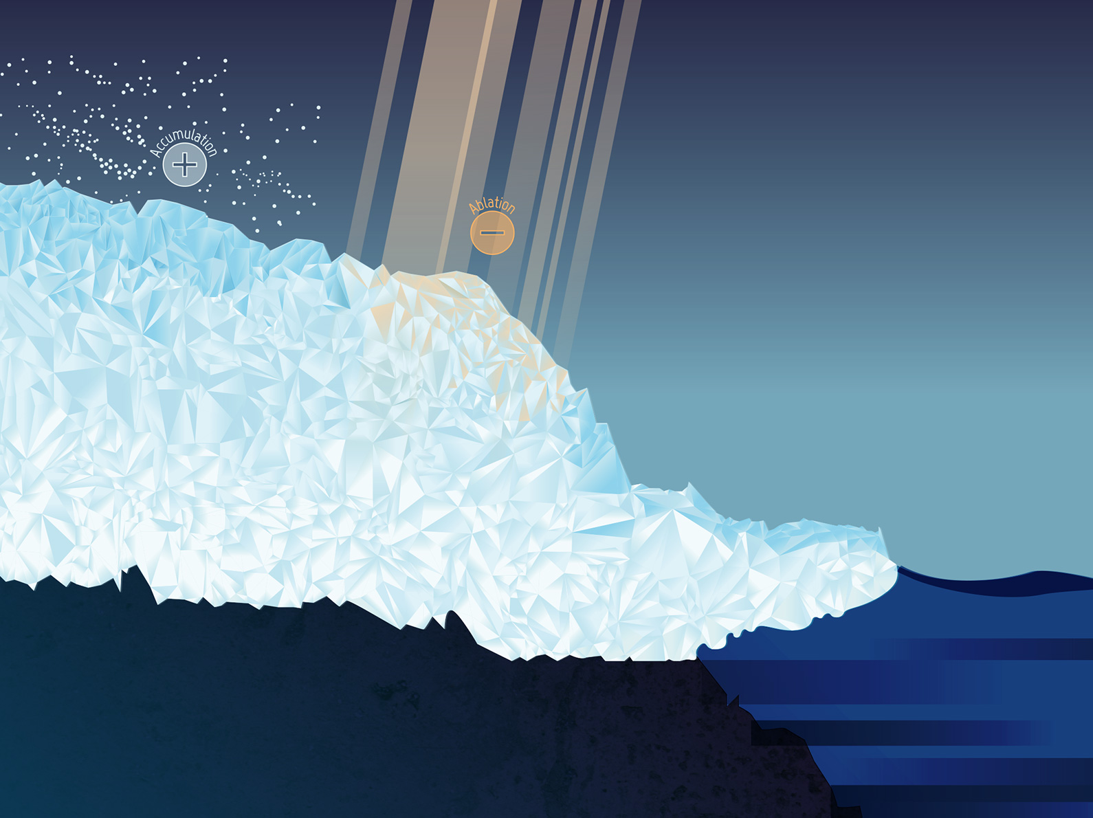
On the surface
On the surface, ice is added to the existing glacier by precipitations and by the refreezing of water: this is accumulation. However, ice also disappears because it melts or because of the wind: this is ablation. The weather conditions and temperature at the surface of the ice cap have an effect on the amount of precipitation as well as on melting and wind transportation, and therefore on accumulation and ablation and consequently on the glacier’s altitude. When the surface temperature increases because of global warming, the ice melts and the altitude decreases through ablation. But the temperature increases when the altitude decreases, so the glacier continues to melt and thin. This phenomenon can therefore escalate and the ice cap can quickly disappear.
This instability of small ice caps is an example of feedback loop, where a cause produces an effect, which in turn has a reinforcing impact on that cause.
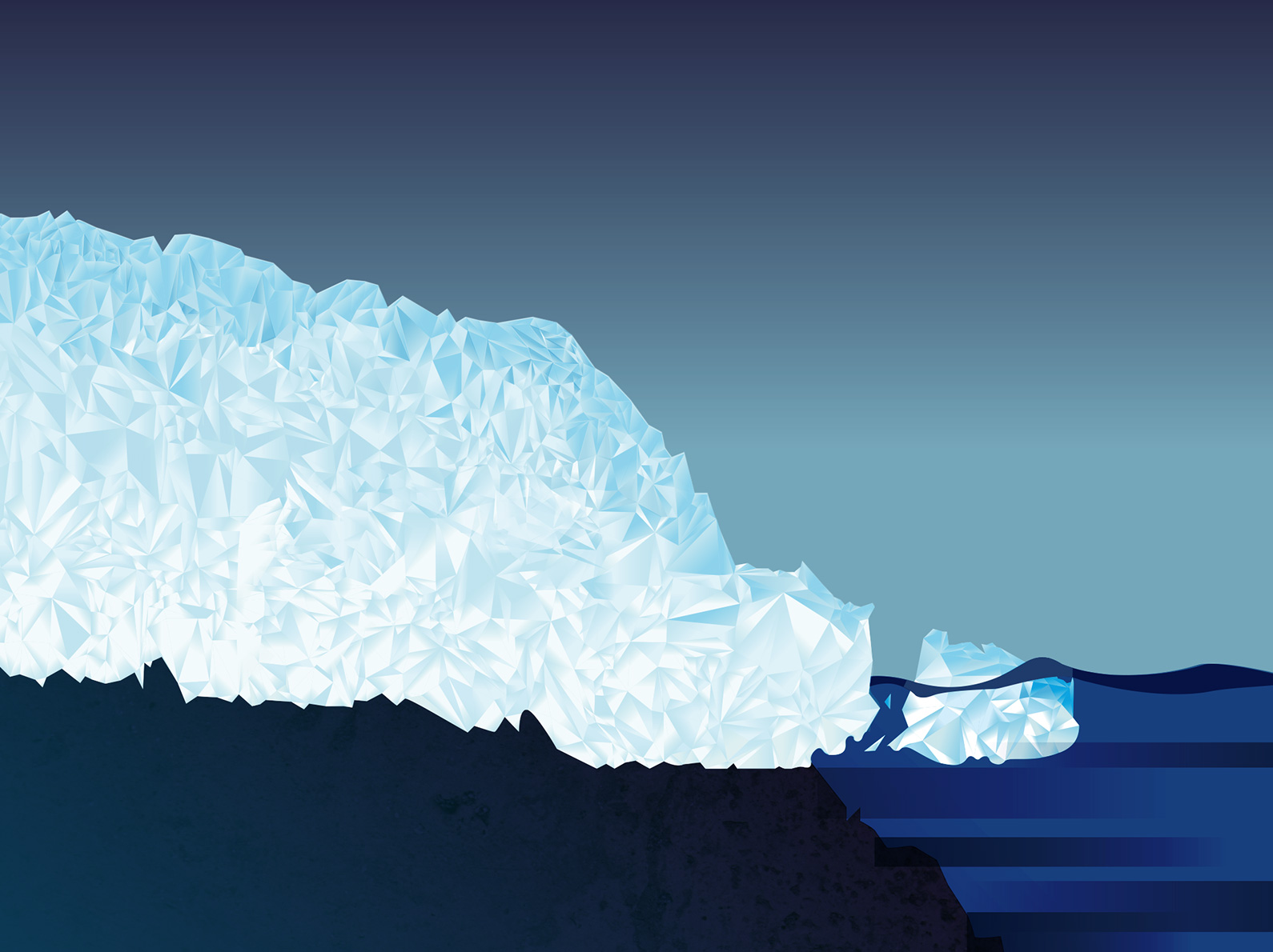
At sea level
Fast outlet glaciers lose large amounts of ice in the form of icebergs and thus contribute to sea level rise. Floating ice shelves are an extension of ice caps over the ocean. When seawater temperature rises, they melt from the base, raising the sea level. This sea level rise in turn affects the velocity of the glacier: feedback can be observed between the different physical processes. The sea level rise changes the grounding line, which is the line where the ice cap starts to float. This modifies the geometry of the ice shelf, and consequently the flow of ice.
Select an area
The mathematical model
Inside
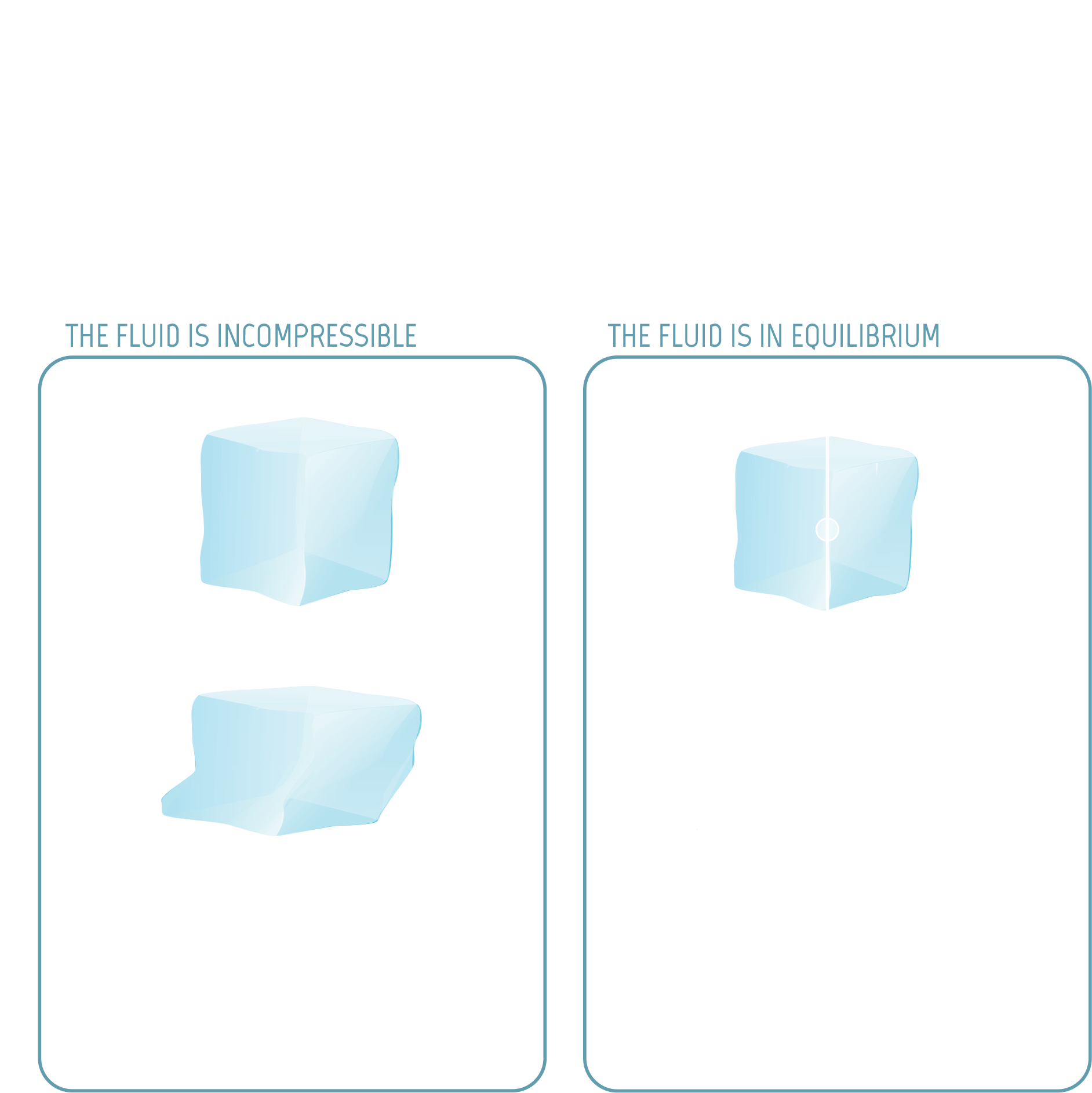
The ice flows because it is a fluid. The model expresses two fundamental laws of physics as equations. On the one hand, the ice is an incompressible fluid, so when a cube of ice changes shape, its volume and mass remain the same: this is the law of conservation of mass. On the other hand, the ice is at equilibrium, so the sum of the forces acting on a cube of ice is zero: this is the law of conservation of momentum, or Newton’s second law, when acceleration is zero.
The forces acting on a cube of ice are due to gravity, pressure and viscosity. To compute the force due to viscosity, a relationship must be defined between the velocity of the fluid and the mechanical stresses due to the plasticity of the fluid. Glaciologists use Glen’s law, which brings temperature into the equation and models the characteristics of the ice crystals.
An equation is also needed to define the temperature inside the ice: this is the law of conservation of energy, which accounts for geothermal flux and surface temperature. In practice, the temperature is often computed separately with a simplified model. Thus a set of equations is obtained in which the unknowns are the velocity of the fluid (intensity and direction) and the pressure, throughout the volume of the glacier. This system of equations is known as the Stokes Equations. They are a simplified version of the notorious Navier-Stokes Equations, for which a 1 million dollar prize has been offered to anyone who can solve them. The Stokes Equations describe the relationships between the variations in velocity and pressure in each direction: they are partial differential equations.
At the base
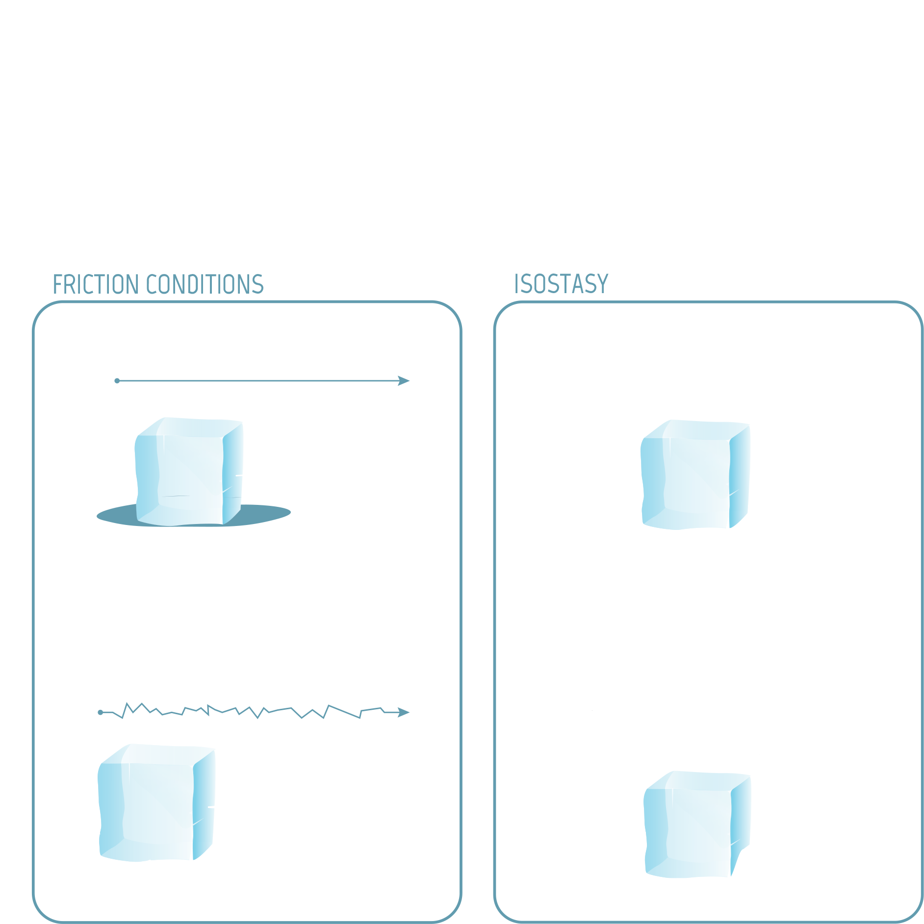
The friction and sliding conditions are complex and are often modelled using a law of friction (another partial differential equation) which involves a friction coefficient specific to the glacier being studied. This coefficient varies in space and is very difficult to measure.
In addition, the altitude of the bedrock can vary. The bedrock slowly sinks under the weight of the ice and slowly rises again when the ice melts. There is feedback between the surface mass balance, the glacier flow, and the altitude of the bedrock. This rebound, known as isostasy, happens after around 10,000 years and can therefore be ignored when changes in the ice sheet over a century are being studied.
On the surface
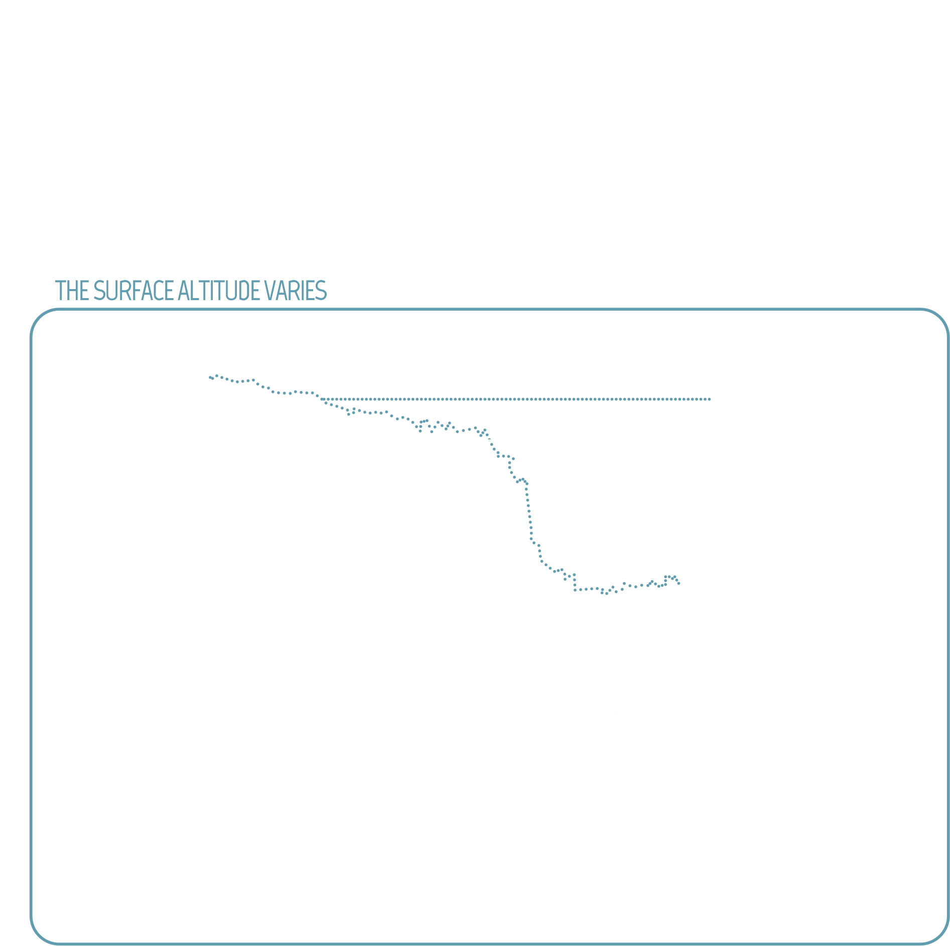
The surface altitude can increase through accumulation or decrease through ablation. It can also vary because of the glacier’s movement. The equation expressing the change over time in the surface altitude is the surface mass balance. Accumulation and ablation are computed using a climate model, while the change due to movement is calculated with the glacier’s surface velocity.
The surface mass balance is also a partial differential equation, with not only spatial variations in the altitude but also variations over time.
At sea level
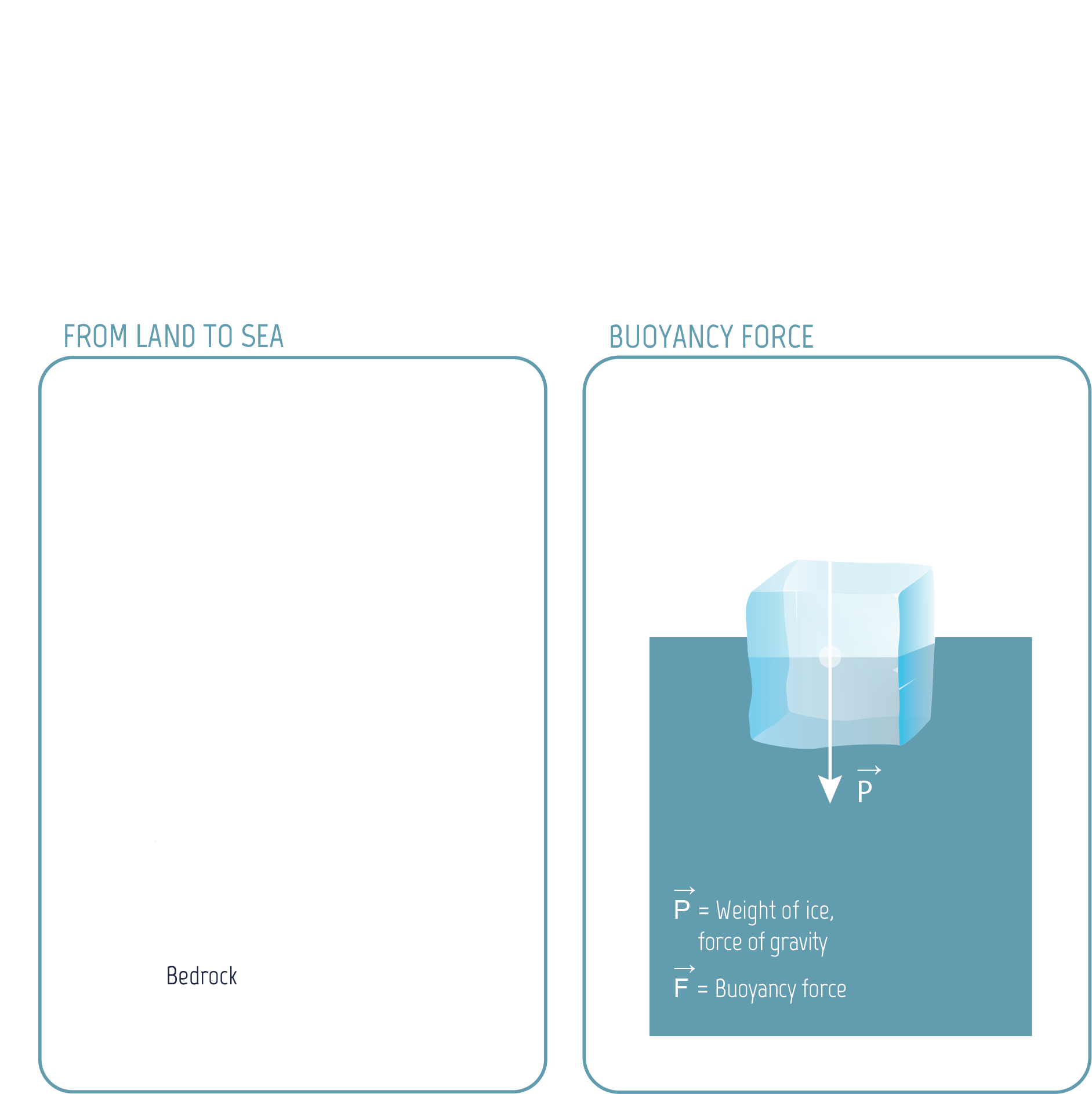
The grounding line is the place where the ice cap starts to float on the ocean. The floating ice shelf is also subject to the buoyancy force exerted by the water. There is an equation expressing the balance of forces for the boundary between the ice cap and the ocean, accounting for the difference in density between ice and water.
There is also an equation for the ice cap’s other boundaries, to complete the system.
Select an area
Computing the ice sheet dynamics
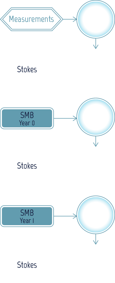
To predict the ice sheet behaviour, it is necessary to compute the surface altitude at regular intervals, e.g. every year. To do this, it is necessary to update the Surface Mass Balance (SMB), which depends on velocity and weather conditions. It is also necessary to adjust the glacier’s velocity, which depends on the altitude.
Since the surface altitude for year 0 is known from measurements, the velocity for year 0 can be computed using the Stokes Equations. The Surface Mass Balance can then be computed for year 0 and the surface altitude for year 1 is worked out from this.
The velocity for year 1 can then be computed, followed by the Surface Mass Balance, and then the surface altitude for year 2, etc.
Computing the velocity of a glacier
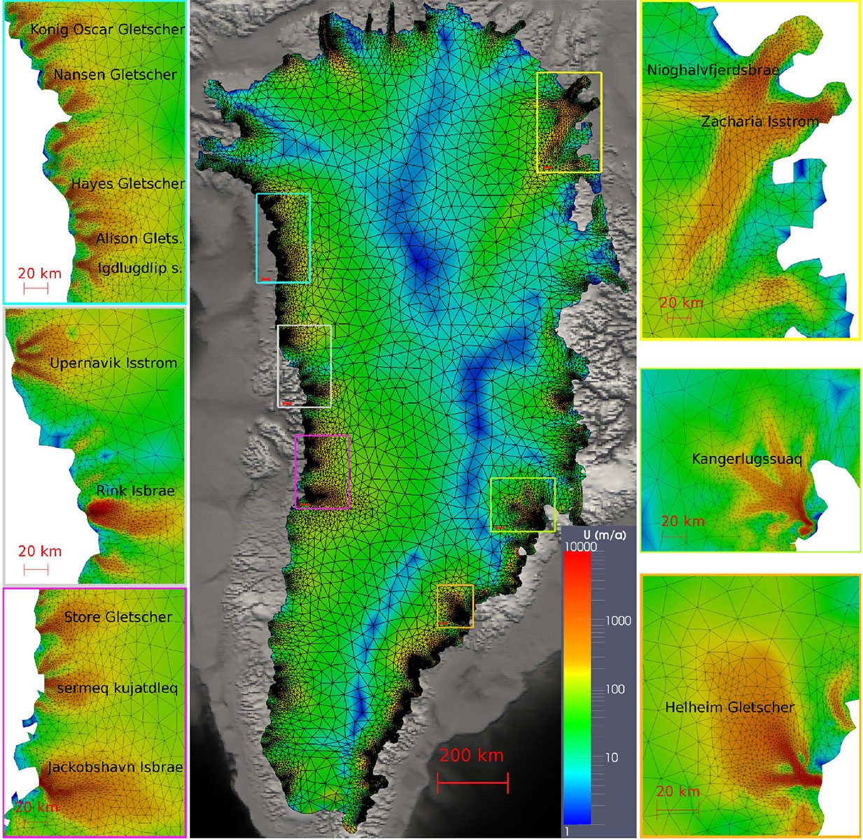
Greenland mesh and simulated velocity. There are more triangles in the outlet glacier areas so that rapid variations in velocity can be computed precisely.
If the surface altitude for year n is known, it is possible to compute the velocity for year n by solving the Stokes partial differential equations.
The first step is to go from unknowns that are everywhere defined to unknowns defined by a finite number of values. This step is known as spatial discretisation. The surface of the glacier is cut up into small triangles, and the thickness of the glacier into slices, which results in the division of the glacier’s volume into prisms (kinds of ice cubes), creating what is known as a mesh.
Image by Gillet-Chaulet, F., Gagliardini, O., Seddik, H., Nodet, M., Durand, G., Ritz, C., Zwinger, T., Greve, R., and Vaughan, D. G.: Greenland ice sheet contribution to sea-level rise from a new-generation ice-sheet model, The Cryosphere, 6, 1561-1576, 2012. Licence CC-BY 3.0.
Solving the stokes equations
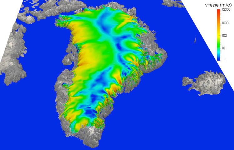
Simulated velocity in 3D of the Greenland ice cap. Outlet glaciers are much faster (in red, 12 km per year) than other areas (in blue, 1 meter per year).
Image by Fabien Gillet-Chaulet, CNRS & LGGE, Grenoble.
The Stokes equations are then converted to a system of complicated algebraic equations (without any derivatives), with as many equations as unknowns. It is not possible to solve exactly such a system; therefore the solution is approximated in a sequence of steps. The iterative algorithm is stopped when a quantity related to the error is small enough.
Quiz
To simulate the ice sheet dynamics, a mesh is defined by cutting the volume into small ice cubes. What happens when the number of ice cubes is reduced?
No, the correct answer is the 2
To compute the velocity and altitude with a good level of accuracy, a high resolution mesh is required, especially in areas of high velocity. But the number of equations increases as the mesh resolution increases and the computation time increases with the number of equations. As with most numerical simulations, a tradeoff has to be found between the accuracy of the result and the computation time.
Bravo!
To compute the velocity and altitude with a good level of accuracy, a high resolution mesh is required, especially in areas of high velocity. But the number of equations increases as the mesh resolution increases and the computation time increases with the number of equations. As with most numerical simulations, a tradeoff has to be found between the accuracy of the result and the computation time.
No, the correct answer is the 2
To compute the velocity and altitude with a good level of accuracy, a high resolution mesh is required, especially in areas of high velocity. But the number of equations increases as the mesh resolution increases and the computation time increases with the number of equations. As with most numerical simulations, a tradeoff has to be found between the accuracy of the result and the computation time.